Assignment 5
Non-photorealistic rendering to transform real images into cartoon-like images
Description
The purpose of this assignment was to explore an application of non-photorealistic rendering; transforming real-life photos into cartoon-like images. I combined this technique with the image alignment from Assignment 1 to transform some images from the Prokudin-Gorskii Collection into cartoon-like images. I also combined the non-phtorealistic rendering technique with the panorama stitching from Assignment 4 to transform the panorama images into cartoon-like panoramas. The technique I used for the cartoon transformation was based off of Holger Winnemoller's paper on Real-Time Video Abstraction.
Algorithm and Implementation
- Convert image from RGB space to LAB space
- Use bilateral filter to smooth within objects
- Convert image from LAB space back to RGB space
- Perform color quantization
- Use Difference of Gaussians to find edges
- Combine filtered, color-quantized RGB image with edges
The Matlab code for this can be found here.
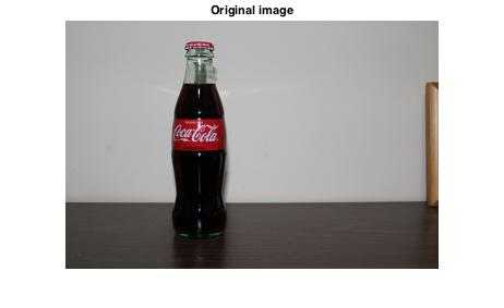
Converting from RGB space to LAB space
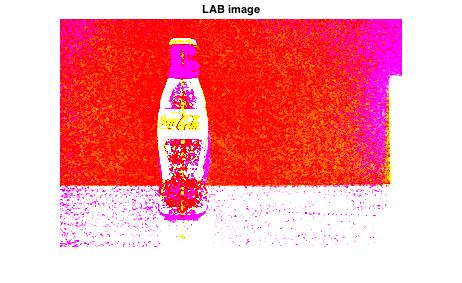
For our past assignments, we've worked primarily in RGB space and occasionally grayscale. As Winnermoller suggested in his paper, I converted my images to LAB space before performing calculations. Similar to RGB space where the image has 3 values for each pixel (red, blue, green), images in LAB space have 3 values for each pixel but these values correspond to luminocity/lightness (L between 0 and 100), red and green component (A between -100 and 100 with -100 being cyan and 100 being magenta), and a yellow and blue component (B between -100 and 100 with -100 being blue and 100 being yellow). I based my code for this conversion off of Yiqun's program on MathWorks.
| Original Image (RGB) |
| LAB Image |
|---|
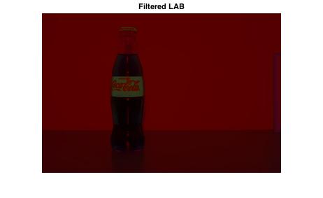
Smoothing with fast bilateral filter
In order to make the image look more cartoon-like I needed to smooth the image while still preserving edges. Winnemoller's paper suggested using a fast bilateral filter to do this. A bilateral filter is a smoothing filter that replaces each pixel's intensity value with a weighted average of intensity values. The calculated value for the pixel depends on the gradients, which allows the filter to preserve edges while still smoothing between edges. A plain bilateral filter is very time costly as it has to compare all pixels to nearby pixels in order to calculate the new intensity values for each location. A fast bilateral filter has been developed that takes significantly less time, and although accuracy is somewhat decreased the time improvement is crucial since we will be performing this filter multiple times for each image. I used Kunal Chaudhury's Matlab code for this section.
| LAB Image |
| Filtered LAB Image |
| RGB Image |
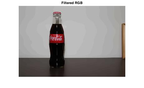
| Filtered RGB Image |
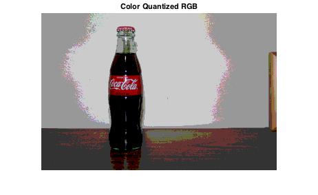
Perform color quantization
Before performing the color quantization, I coverted the filtered LAB image back to RGB space. In Winnemoller's paper, he performed the color quantization on the lumosity channel of the LAB image, but I had better results when converting to RGB and using the three color channels. This is perhaps due to the way I performed the color quantization. I used Matlab's rgb2ind function which converts an image to an indexed image with fewer colors. Specifically, it takes a number between 0 and 1.0 as an input and restricts the number of colors in the output image to (floor(1/inputNumber)+1)^3.
| Filtered RGB Image |
| Color Quantized RGB Image |
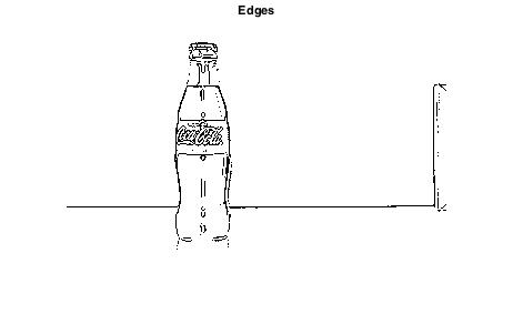
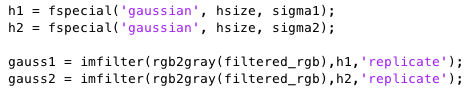
Use Difference of Gaussians to find edges
I used difference of Gaussians from the Lecture 14 slides to perform the edge detection on my image. I chose a standard deviation of 0.375 and 0.2625 for the two smoothed images as those seemed to provide the best edges. After obtaining the edges I used Matlab's medfilt2 function to perform 2-D median filtering, which got rid of some isolated edges that were causing noise.
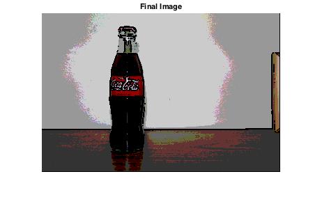
Combine edges with color-quantized smooth image
The final step was simply adding the edges onto the smoothed RGB image. The values for my edges image were 0:255 so I set a threshold of 200 and set all pixels in the final image equal to zero if the corresponding pixel in the edges image was below the threshold.
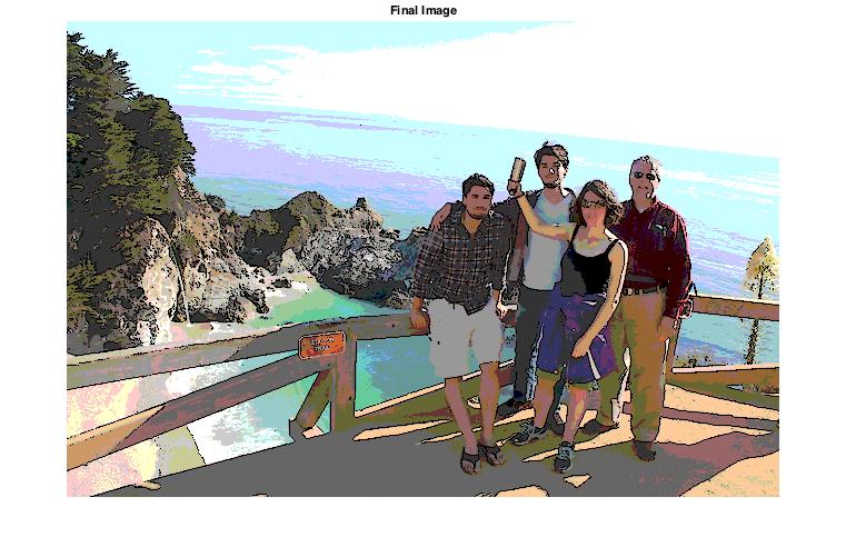
| Original Image |
| Final Image |
Results
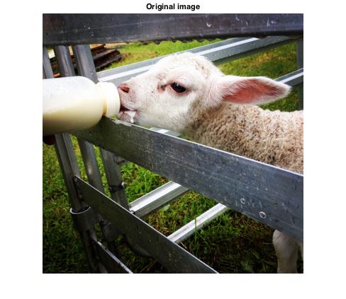
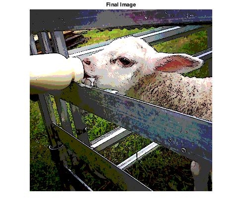
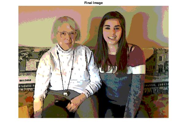
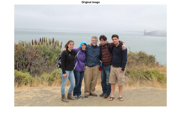
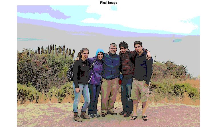
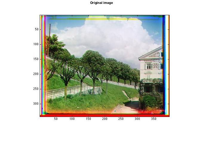
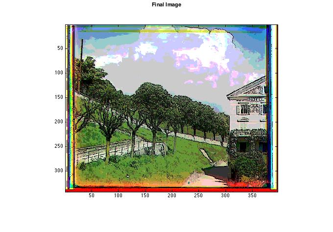
| Original Image |
| Final Image |
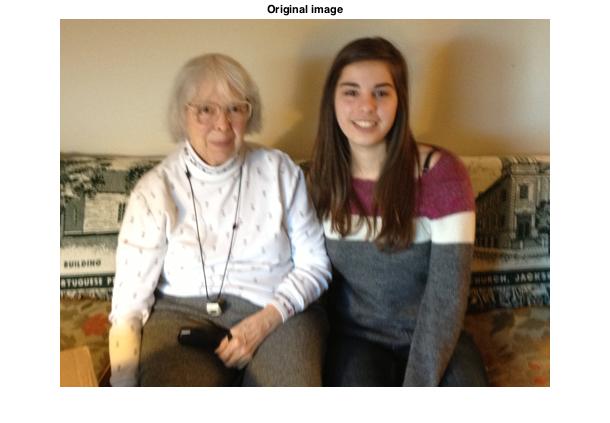
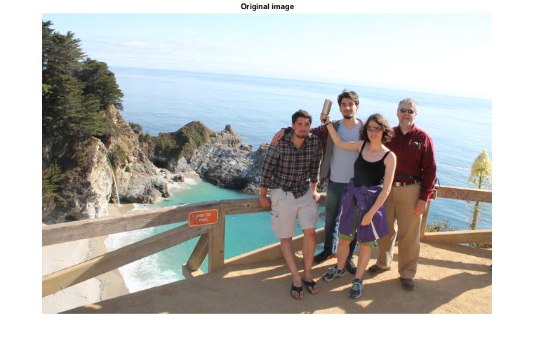
| Original Image |
| Final Image |
| Original Image |
| Final Image |
| Original Image |
| Final Image |
| Original Image |
| Final Image |
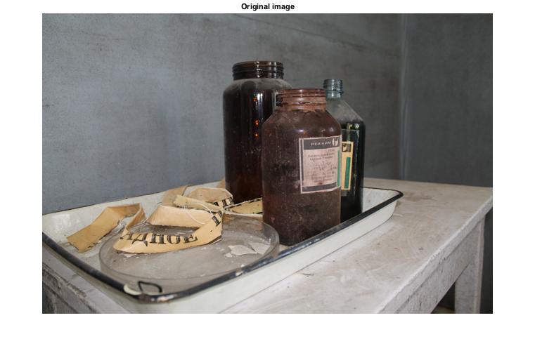
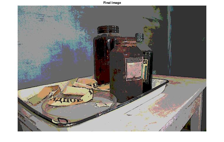
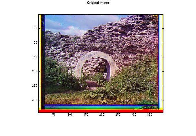
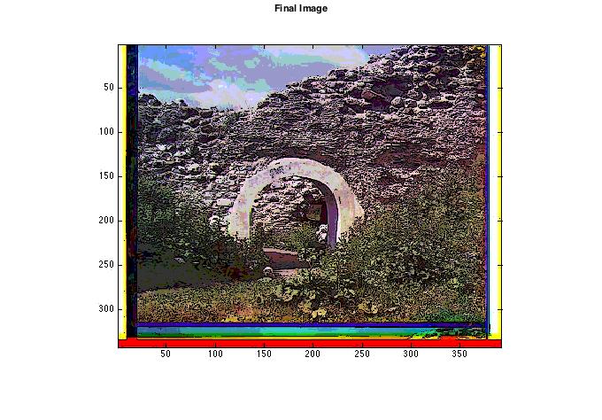
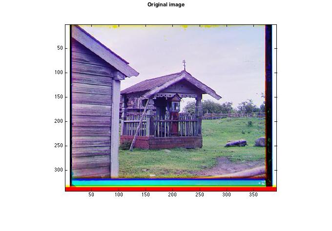
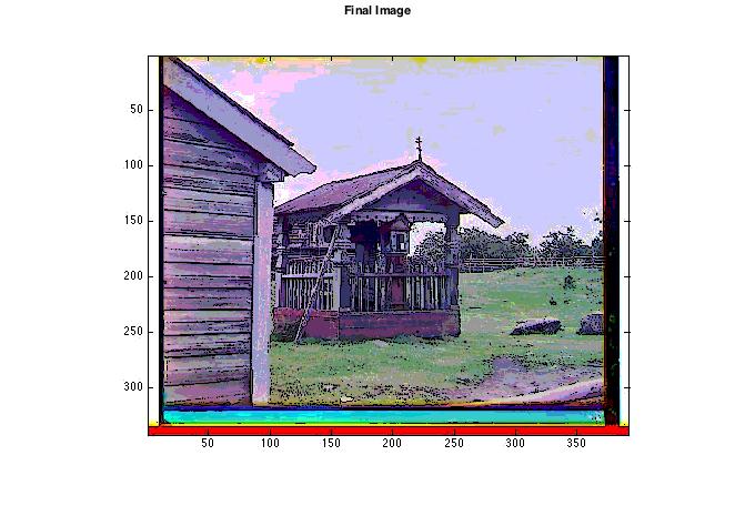
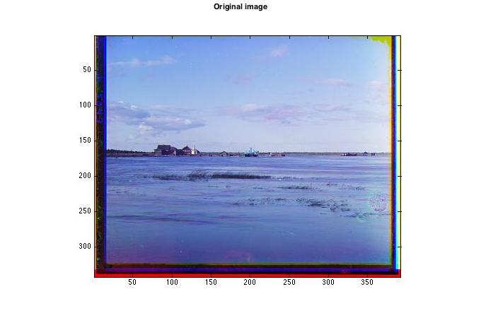
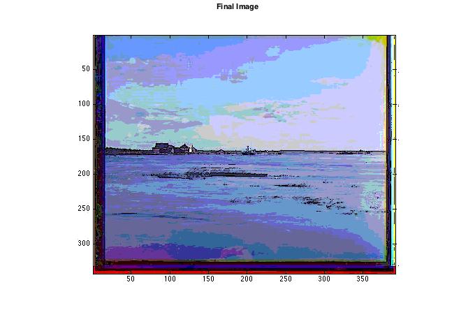
Results using images from Prokudin-Gorskii Collection after alignment
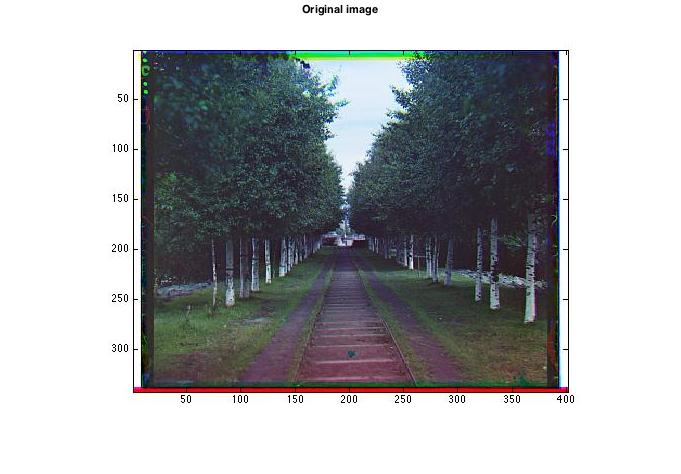
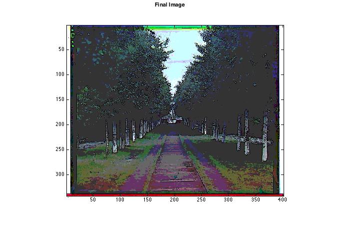
| Original Image |
| Final Image |
| Original Image |
| Final Image |
| Original Image |
| Final Image |
| Original Image |
| Final Image |
| Original Image |
| Final Image |
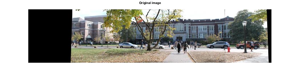
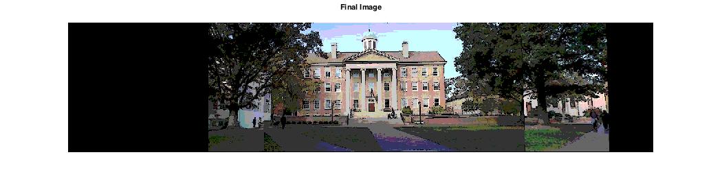
Results using panorama images
Original Image |
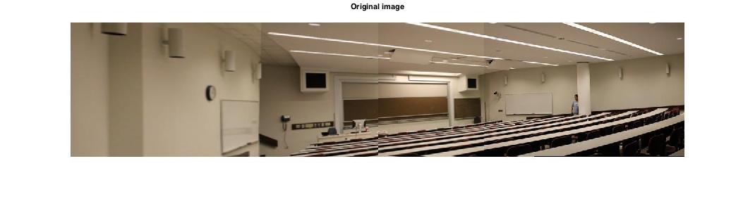 |
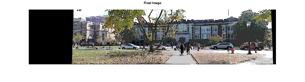
Final Image |
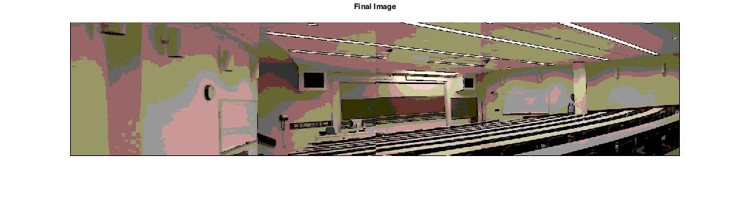 |
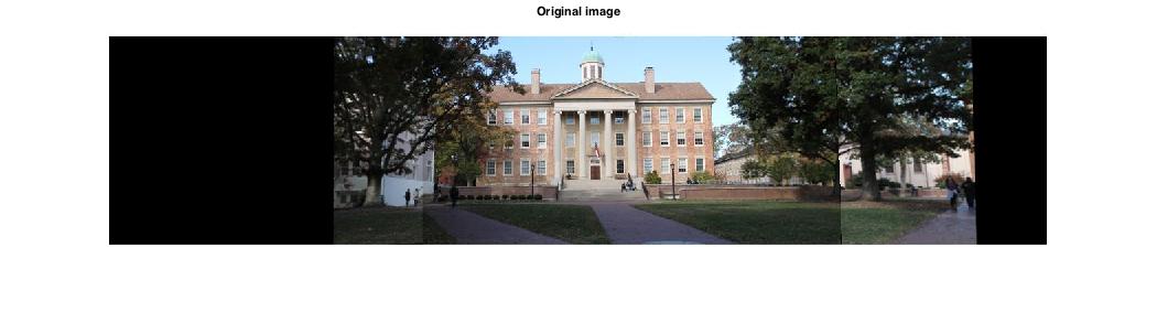
Original Image |
 |
Final Image |
 |
Original Image |
 |
Final Image |
 |
Discussion
There were a number of parts of this project that I did differently than Winnemoller, which could account for the difference in quality of results. While my results were successful, I do think his methods provided a slight improvement over mine. One of the differences between my algorithm and Winnemoller's was the color quantization step. Winnemoller performed the color quantization on the luminance (L) channel in LAB space and converted back to RGB after performing the color quantization. I chose to perform the color quantization in RGB space because the Matlab function I used was only applicable to RGB images, but I seemed to get fairly effective results even with this adjustment.
Another adjustment I made was in the edge detection step. Winnemoller chose to use Difference of Gaussians with a slightly smoothed step function with the following formula:
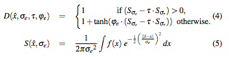
Rather than using this formula, I used the following Matlab function:
This change in edge detection contributed to some of the differences between my results and the results in Winnemoller's paper, though my edge detection method was still successful in retrieving the important edges in my images.
Website design by Yipin Zhou.